Polaris
Introducing Polaris-4B-Preview and Polaris-7B-Preview, the most powerful open-recipe reasoning models to date.
POLARIS: A POst-training recipe for scaling reinforcement Learning on Advanced ReasonIng modelS
Team: Chenxin An *, Zhihui Xie†, Xiaonan Li†, Lei Li†, Jun Zhang, Shansan Gong, Ming Zhong
Jingjing Xu *, Xipeng Qiu, Mingxuan Wang, Lingpeng Kong
*: Project Leads; †: Significant Contributor
Affiliations: The University of Hong Kong, Bytedance Seed, Fudan University
We are thrilled to unveil our latest breakthroughs, POLARIS-7B-Preview and POLARIS-4B-Preview, which mark a new frontier in open‐recipe reasoning models developed using academic‐level resources. POLARIS-4B-Preview is fine-tuned from Qwen3-4B and POLARIS-7B-Preview is fine-tuned from Deepseek-R1-Distill-Qwen-7B. Our 4B model achieves an impressive 81.2% Pass@1 accuracy on AIME24 and 79.4% Pass@1 accuracy on AIME25, outperforming state-of-the-art commercial models like Claude-4-Opus, Grok-3-Beta, and o3-mini-high(2025/01/31) via scaling reinforcement learning on open-source data. On AIME25, POLARIS astonishingly achieves comparable performance to Qwen3-235B-A22B while using less than 2% of its parameters and can be deployed on consumer-grade GPUs.
To foster progress in scaling RL on advanced reasoning models, we are open-sourcing our dataset, code, and training details for the research community.
👨💻 Github | 🤗 HF Model | 🤗 HF Dataset | 📖 paper | 🔎 Evaluation results
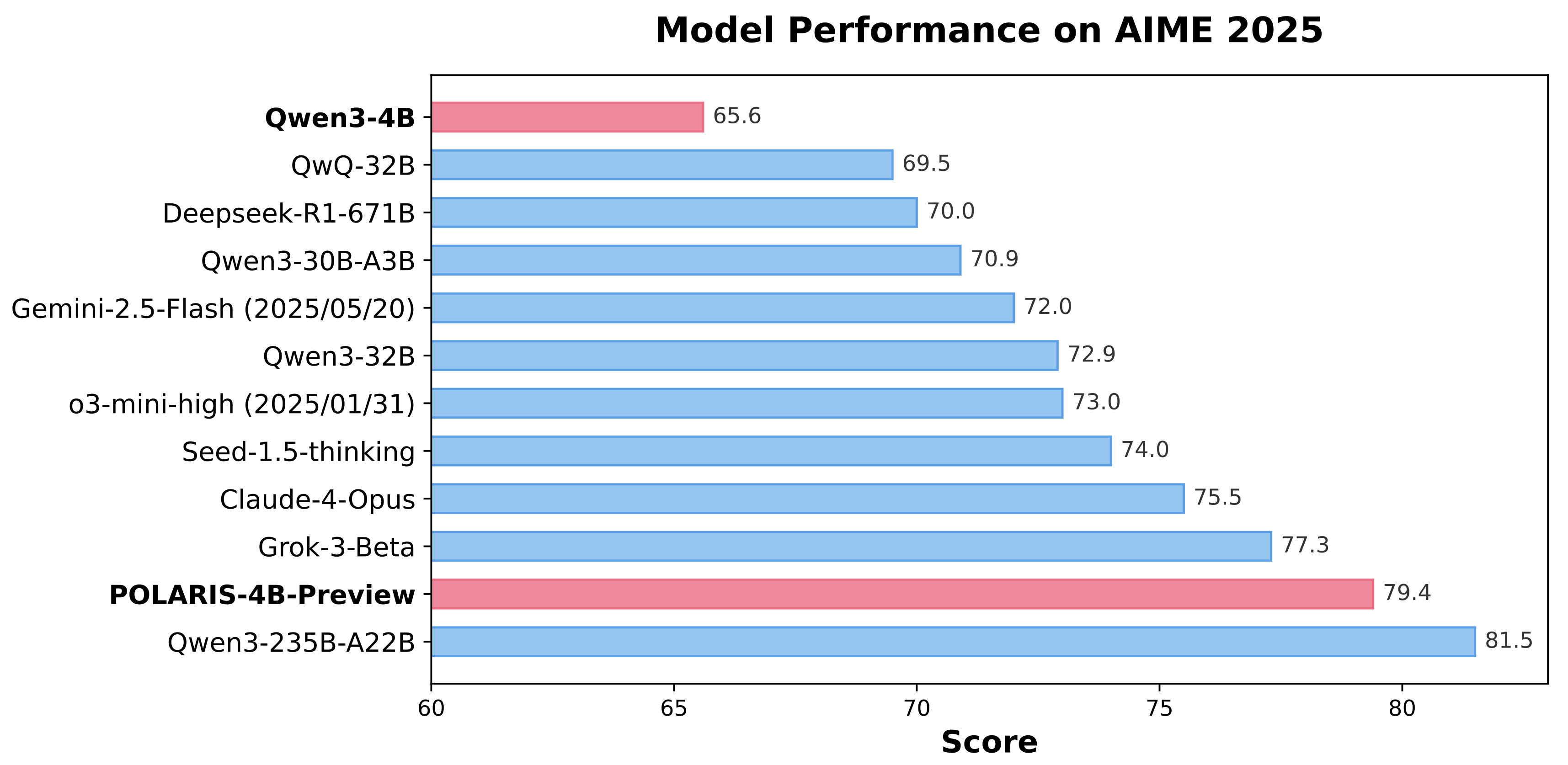
✅ Takeaways for post-training of advanced reasoning models
Data Difficulty: Before training, Polaris analyzes and maps the distribution of data difficulty. The dataset should not be overwhelmed by either overly difficult or trivially easy problems. We recommend using a data distribution with a slight bias toward challenging problems, which typically exhibits a mirrored J-shaped distribution.
Diversity-Based Rollout: We leverage the diversity among rollouts to initialize the sampling temperature, which is then progressively increased throughout the RL training stages.
Inference-Time Length: Polaris incorporates length extrapolation techniques for generating longer CoT at inference stage. This enables a "train-short, generate-long" paradigm for CoT reasoning, mitigating the computational burden of training with excessively long rollouts.
Exploration Efficiency: Exploration efficiency in Polaris is enhanced through multi-stage training. However, reducing the model's response length in the first stage poses potential risks. A more conservative approach would be to directly allow the model to "think longer" from the beginning.
POLARIS’s Recipe
Current work (e.g., DeepscaleR) demonstrates that a small model (e.g., 1.5B parameters) can achieve surprising improvements in reasoning tasks through scaling RL training. However, when we apply their recipe to train more advanced reasoning models, we observe marginal improvements even decline during the RL training of Qwen3. This suggests a critical gap in the open-source community’s understanding of how to further scale RL on advanced reasoning models. To address this, we introduce POLARIS—a post-training recipe centered on calibrated data difficulty, enhanced data diversity, inference-time length scaling, and efficient training.
We are committed to transparency and will be open-sourcing our trained models, training code, and data to foster community progress.
1. Data Difficulty
Our POLARIS recipe builds upon a deep investigation on the training data difficulty. Specifically, we conduct controlled experiments regarding data difficulty measured by model pass rate, and choose public available training datasets to enable better reproducibility.
Balanced Data Difficulty Matters
Our initial experiments involve training models of different scales on the public DeepScaleR dataset. While a 1.5B model shows significant performance gains as expected, a 7B model trained on the same data exhibits only marginal improvements. We observe that the 7B model’s average reward quickly surpasses 0.7, indicating that the training set is too simple to drive further improvements.
This leads us to a core hypothesis: For effective RL training, the difficulty of the data must be carefully calibrated to the model’s scale and capability.
To validate this, we analyze the difficulty distribution of the 40,000 samples in the DeepScaleR training set. We use Deepseek-R1-Distill-Qwen-7B and its 1.5B version to perform an offline evaluation, generating 8 solutions for each problem with a sampling temperature of 0.6. The percentage of correct solutions serves as a proxy for the difficulty of each sample.
The results, shown in the figure below, are revealing.
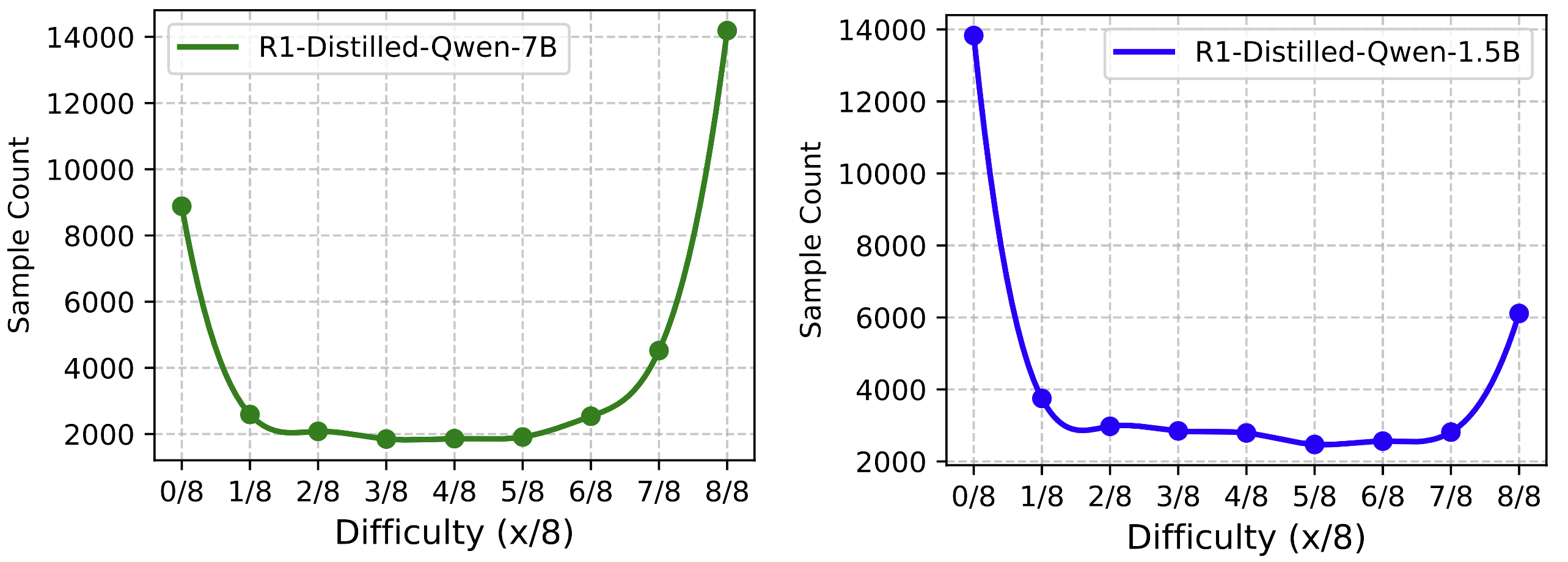
Across both model scales, we observe that most problems are either very easy (8/8 correct solutions) or very hard (0/8 correct solutions). Crucially, we note a “mirror effect” between the two models:
- The 1.5B model shows a mirrored J-shaped (Ⴑ) distribution, with most problems being extremely difficult (0/8 correct).
- The 7B model shows a standard J-shaped distribution, with the vast majority of problems being far too easy (8/8 correct).
This stark contrast confirms that the dataset, while challenging for a 1.5B model, is not sufficiently difficult to train a 7B model effectively. This insight motivates our work in curating a new, more challenging dataset tailored for advanced models.
To confirm our hypothesis, we conduct an ablation study on the DeepScaleR 40K dataset using the Deepseek-R1-Distill-Qwen-7B model. We create distinct training sets by systematically altering the difficulty distribution:
- Full Dataset (40K samples): The dataset exhibits the original J-shaped distribution, dominated by easy samples (8/8 correct solutions).
- Removal of Perfect Scores (26K samples): We remove all samples with 8/8 correct solutions, creating a mirrored J-shaped distribution.
- Aggressive Filtering (19K samples): We filter out all samples with a pass rate greater than 4/8, resulting in an distribution that focuses only on the hardest problems.
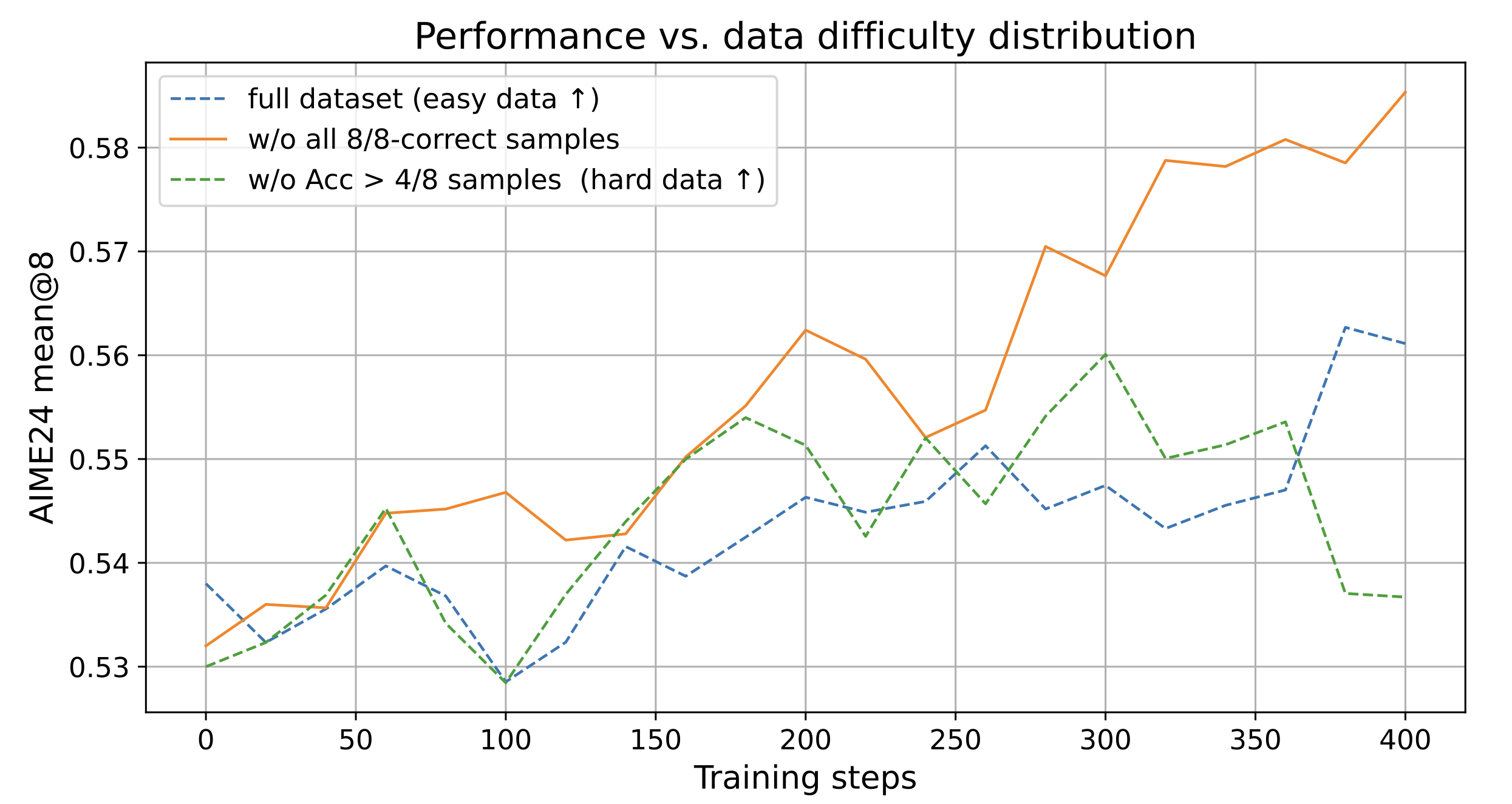
The results, as shown in Figure 1, clearly demonstrate that removing the easiest samples leads to consistent performance improvements. In contrast, both the unfiltered dataset (which lacks sufficient challenge) and the aggressively filtered dataset (which is overly saturated with difficult problems) hinder training progress.
These findings confirm that optimal RL training requires a balanced difficulty distribution—one that provides enough challenging samples to drive learning while avoiding both trivial problems and overwhelming difficulty.
POLARIS’s Data Curation Strategy
Motivated by these findings, the POLARIS recipe curates a mirrored J-shape difficulty distribution by filtering high-quality public datasets, including DeepScaleR-40K, and AReaL-boba-106k.
Our data engineering process is as follows:
- Offline Difficulty Estimation: We use the specific model being trained to generate
8 rolloutsfor each potential training problem. The pass rate determines the problem’s difficulty relative to that model. - Targeted Filtering: To create the desired mirrored J-shape distribution, we remove all samples that the model solves perfectly (8/8 correct).
- Dataset Assembly and Calibration:
- For training
Deepseek-R1-Distill-Qwen-7B, we applied this filtering to DeepScaleR and AReaL, creating a final training set of 53K samples (26K from DeepScaleR and 27K from AReaL). - To train the the
Qwen3-4Bmodel, we performed an additional filtering pass on this 53K set, resulting in a 30K sample dataset specifically calibrated to its difficulty level.
- For training
This model-specific calibration of data difficulty is a cornerstone of the POLARIS recipe, ensuring that the training process remains challenging and effective for any given model.
Dynamically drop easy data during training
As the RL training process progresses, the model’s capabilities will grow, and the proportion of difficult questions will decrease. Therefore, in addition to initially adjusting the difficulty distribution, we also adjust the training data distribution during the training process. Here is the figure showing the distribution shift of data difficulty during training.
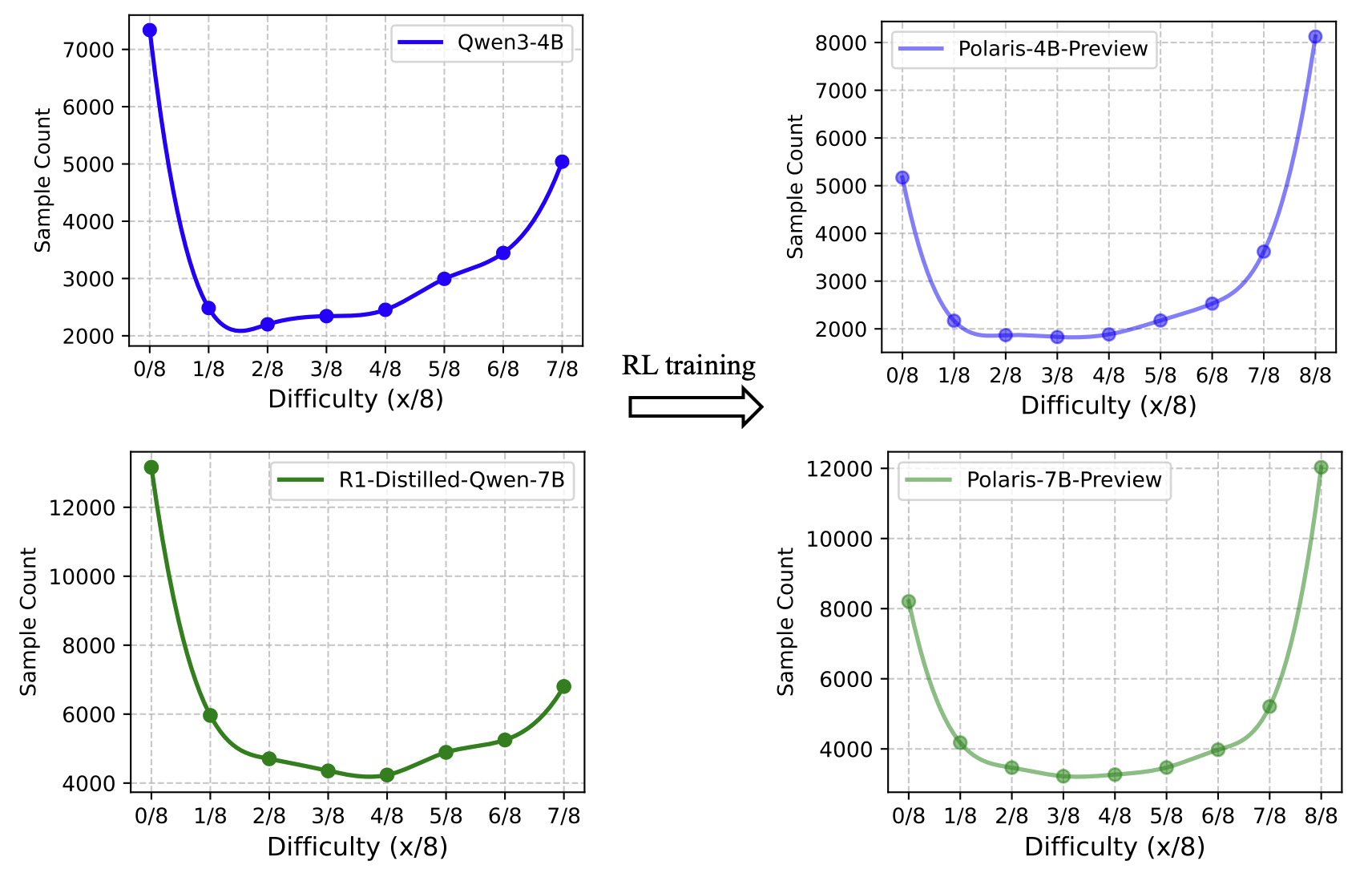
We observe that the sample difficulty distribution consistently shifts from a mirrored J-shape (Ⴑ) to a J-shape. This evolution reinforces our motivation to start with a Ⴑ-shaped distribution, allowing for a smooth transition to the J-shape.
Additionally, since data difficulty changes dynamically during training, using the initial dataset throughout is suboptimal. To maintain an ideal difficulty distribution, we introduce dynamic difficulty distribution updates: during training with a rollout size of n=8, we update each sample’s accuracy after reward computation (initial difficulty determined by offline filtering accuracy). At the end of each training phase, we remove samples with Accuracy > 0.9 to preserve the initial distribution shape and prevent skewing towards a J-shape.
This dynamic filtering ensures that the model continues to face appropriately challenging samples, preventing the learning signal from degrading due to an overabundance of mastered samples.
2. Diversity-based Rollout Sampling
In GRPO training, diversity is an essential factor. GRPO’s key is to contrast positive and negative trajectories, increasing the probability of positive ones. The diversity of sampled trajectories is crucial, encompassing two aspects:
- High diversity encourages the model to generate both positive and negative trajectories in a single rollout, enhancing trajectory contrast.
- High diversity allows the model to explore a wider range of potential reasoning paths, which helps prevent the model from quickly becoming overconfident in a narrow set of patterns. We also explore the method to increase the sampling diversity. Our approach aims to achieve the best diversity while ensuring performance.
During the rollout phase, the primary hyperparameters affecting diversity are top‑p,top‑k, and the sampling temperature. In previous open‑source projects, the default settings are typically a top‑p value of 1.0 and a top‑kvalue of –1, which together yield maximum diversity. Only the sampling temperature remains adjustable. Temperature is usually established either by following the decoding temperature recommended on the official website (e.g., 0.6) or by setting it as a hyperparameter at 1.0. Therefore, in this section, we focus on temperature to analyze how the temperature affects the RL training performance and propose adjusting the temperature during training to match the base model’s diversity.
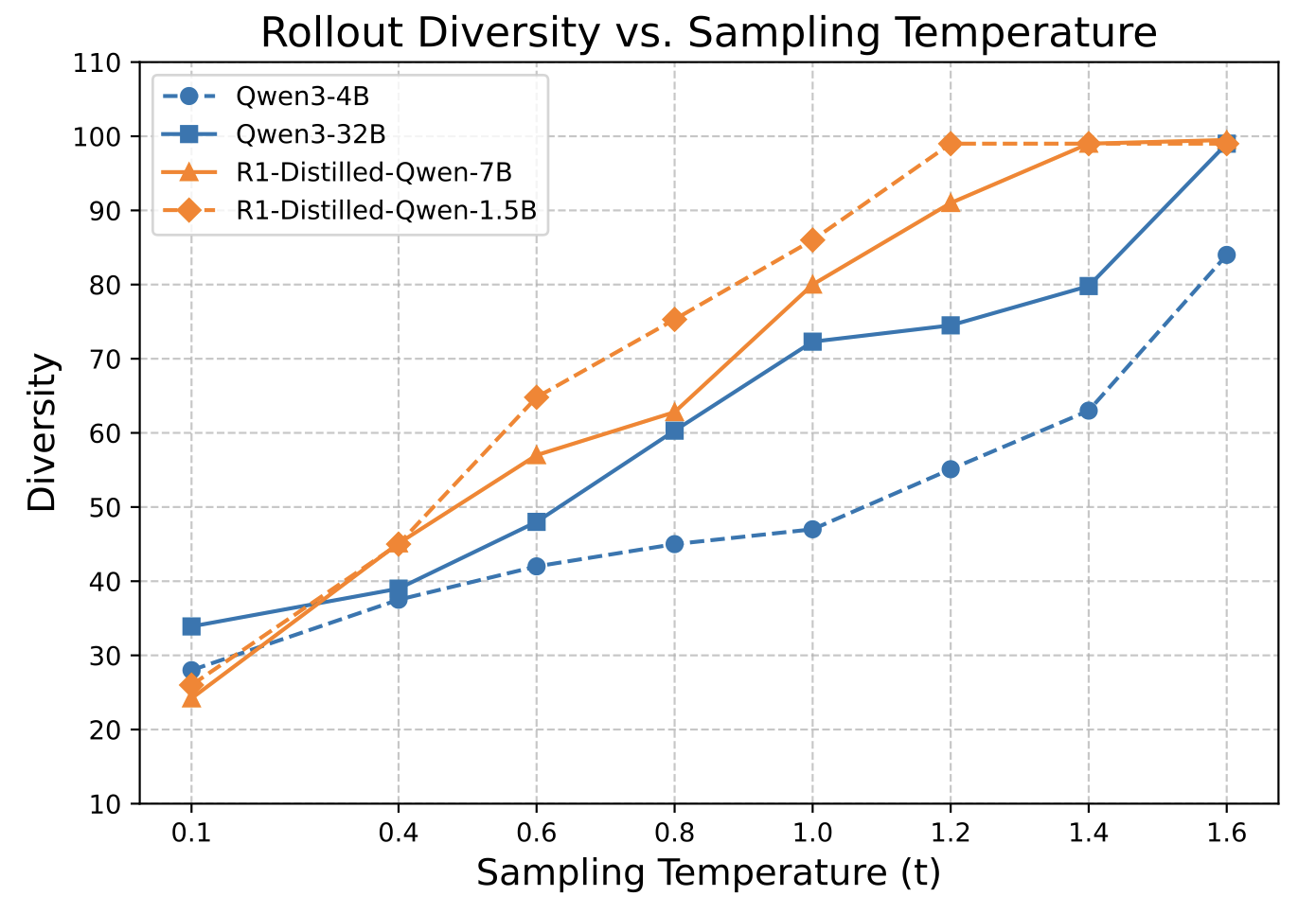
We start from a probing experiment to explore the relationship between sampling temperature $t$, performance (mean@32), and diversity among rollouts. To quantify the diversity of the sampled trajectories, we use the distinct N-gram metric. This metric evaluates lexical diversity by measuring the ratio of unique N-grams (contiguous sequences of n words) to the total number of N-grams across all generated outputs. In our experiments we set N=4. A score closer to 1.0 indicates higher diversity, meaning the all trajectories contain a wide variety of phrases with little repetition. Conversely, a score closer to 0 indicates low diversity, suggesting the generated outputs are highly similar or repetitive.
Diversity vs. Sampling Temperature: Higher temperatures bring better diversity. To use more diverse trajectories for training, it is recommended to increase the sampling temperature. At the same temperature, there are significant differences in diversity performance across models. For instance, Qwen3 has fewer unique n-grams and a more concentrated output distribution.
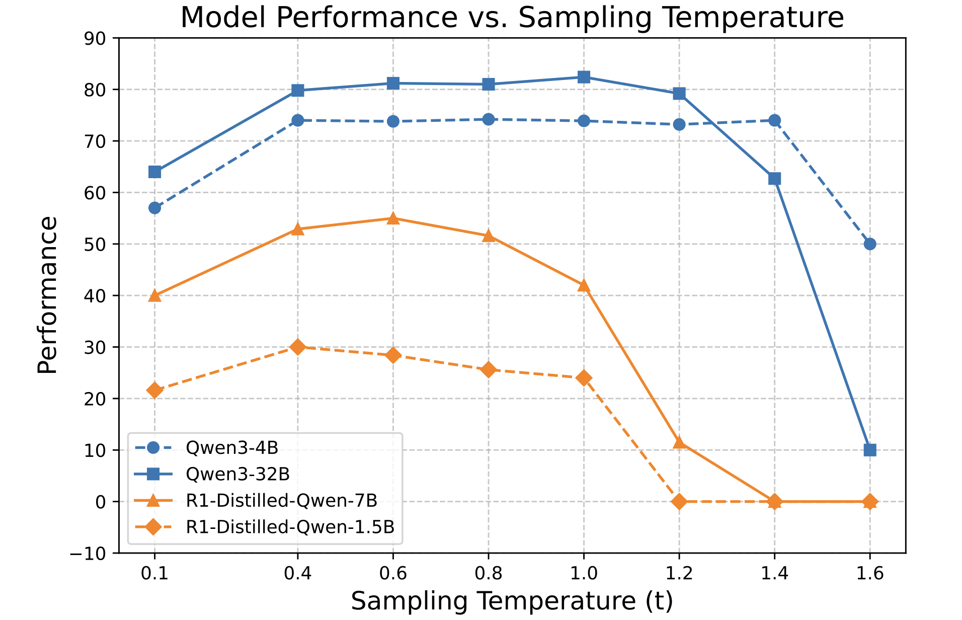
Performance vs. Sampling Temperature: While pursuing diverse trajectories, it is also necessary to ensure the model’s performance. When we increase the temperature from 0 to higher, all the tested models’ average accuracy exhibits a low-high-low trend. We also notice that each model has significant differences in their zone spans, highlighting that there is no one-size-fits-all temperature setting . The optimal temperature for achieving a desired level of diversity is highly dependent on the specific model being used.
Definition: Temperature Zone
According to the trends, we can get the following sampling temperature zone empirically:
- Robust Generation Zone (RGZ): RGZ defines the zone where the model’s performance is both
optimalandstable, without significant increases or decreases. The suggested decoding temperature is typically from RGZ. - Controlled Exploration Zone(CEZ): Temperature in CEZ leads to slight performance degradation compared with RGZone, but the degradation level is acceptable because it leads to the increased rollout diversity.
- Performance Collapse Zone (PCZ): In PCZ, the model tends to output noisy tokens and thus the performance will be extremely low.
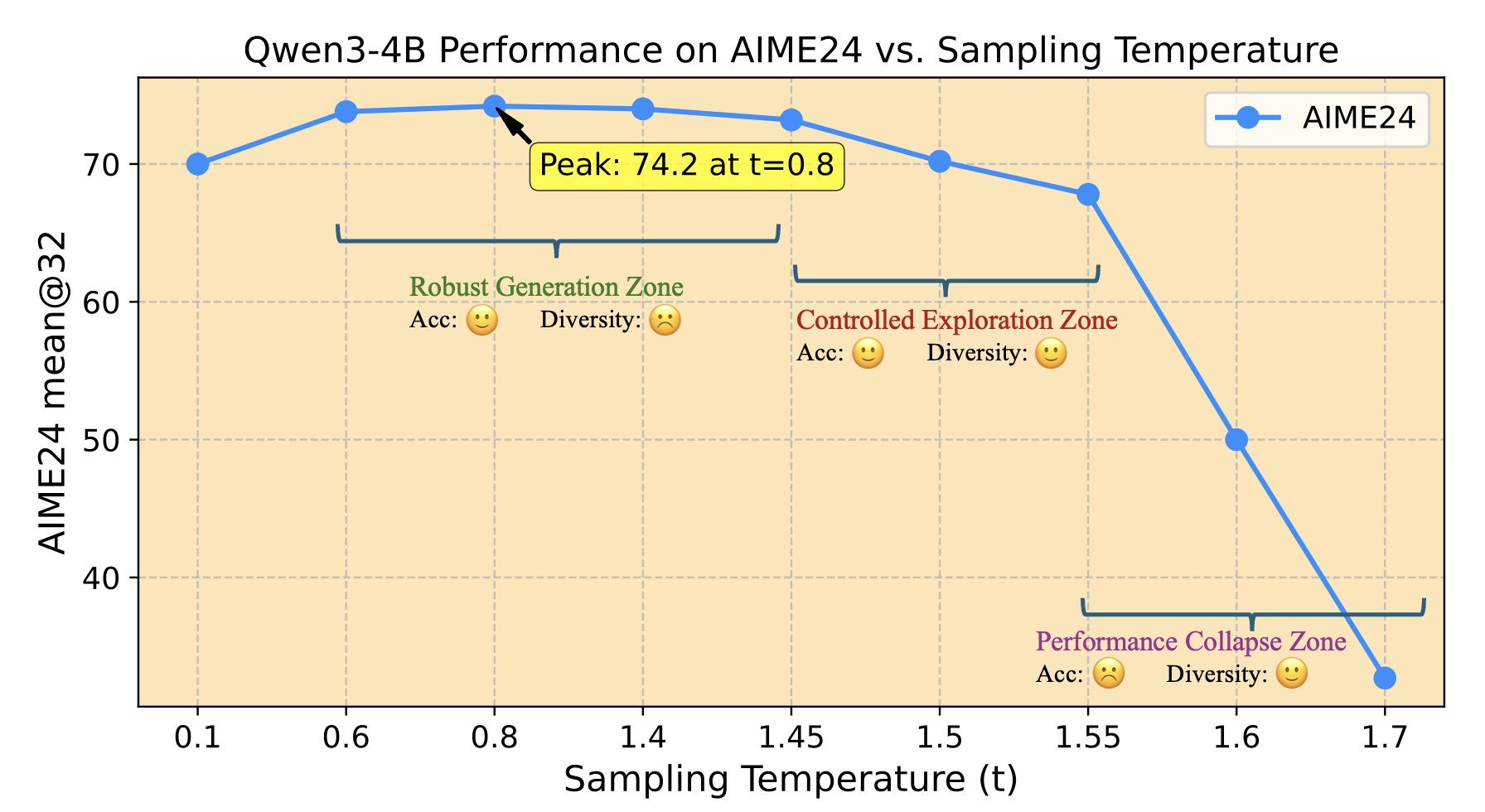
For illustration, We show Qwen3-4B’s accuracy on AIME24 to demonstrate the differences among these three areas in the following figure. When temperature is 0.6~1.4, the model achieves the optimal and stable performance curve. When temperature is 1.4-1.55, the performance slightly degrades but has better rollout diversity. Then increasing temperature from 1.55 to 1.7 causes significant model performance collapse, which indicates the PCZone starts from temperature=1.55. Noise begins to appear, making it unsuitable for both training and decoding.
Temperature initialization on Controlled Exploration Zone
Our probing experiments reveal that sampling temperature significantly impacts rollout diversity, and its optimal setting varies across base models. The recommended test temperatures are usually from Robust Generation Zone , which usually result in low diversity. An overly deterministic sampling temperature restricts the model’s ability to explore better pattern spaces. In Polaris, we propose initializing the sampling temperature based on the model’s Controlled Exploration Zone to achieve comparable performance with improved diversity.
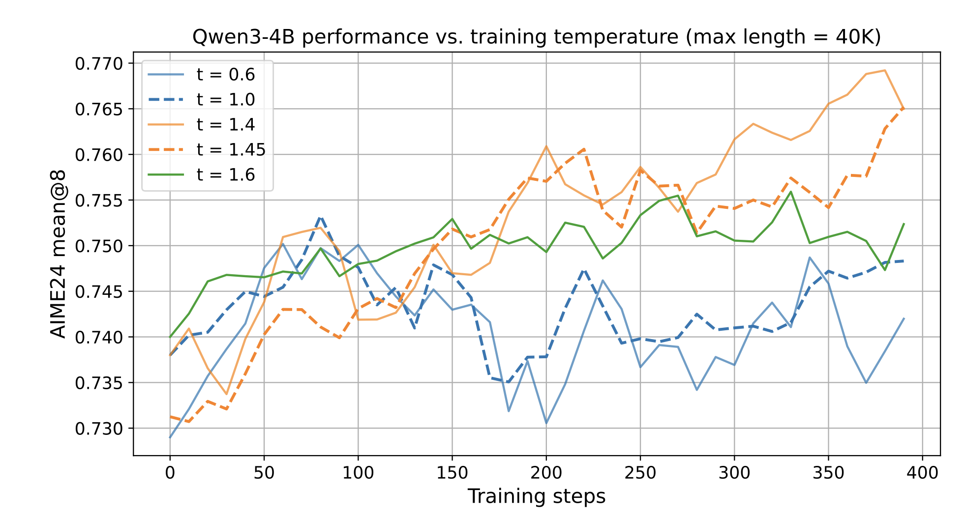
We recommend using the sampling temperature at the point where model performance begins to decline while maximizing diversity. For Qwen3-4B and Deepseek-R1-Distill-Qwen-7B, we set the initial sampling temperatures to 1.4 and 0.7, respectively.
The comparison of different temperature initialization settings shows that the most common setting, t= 0.6 / 1.0, causes a decline in model performance, as it is too low to allow the model to explore better trajectories. In contrast, the temperature within the Controlled Exploration Zone demonstrates the best RL performance.
Dynamic Temperature Reset Across Training Stages
We also find that the model’s Robust Generation Zone and Controlled Exploration Zone shift during RL training (as shown in the following figure). Since reinforcement learning increases the probability of positive expression patterns, the model’s entropy tends to decrease and its exploration space becomes narrower, which is manifested by the convergence of N-grams in different trajectories.
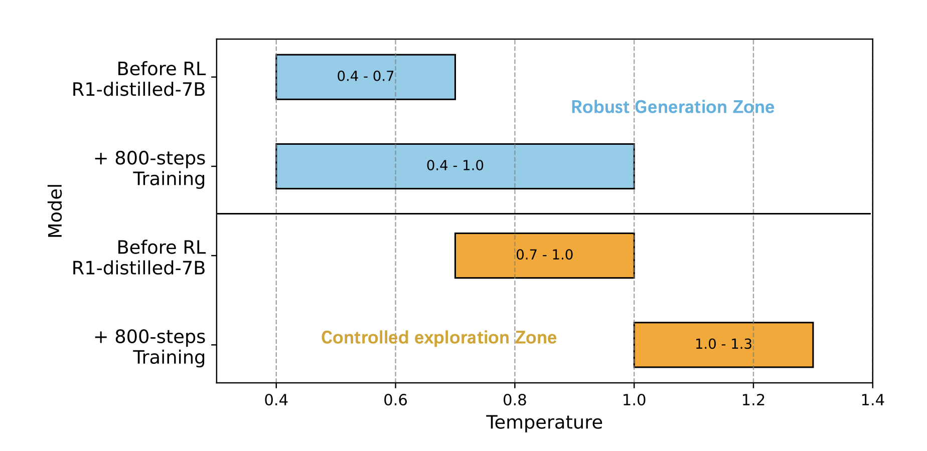
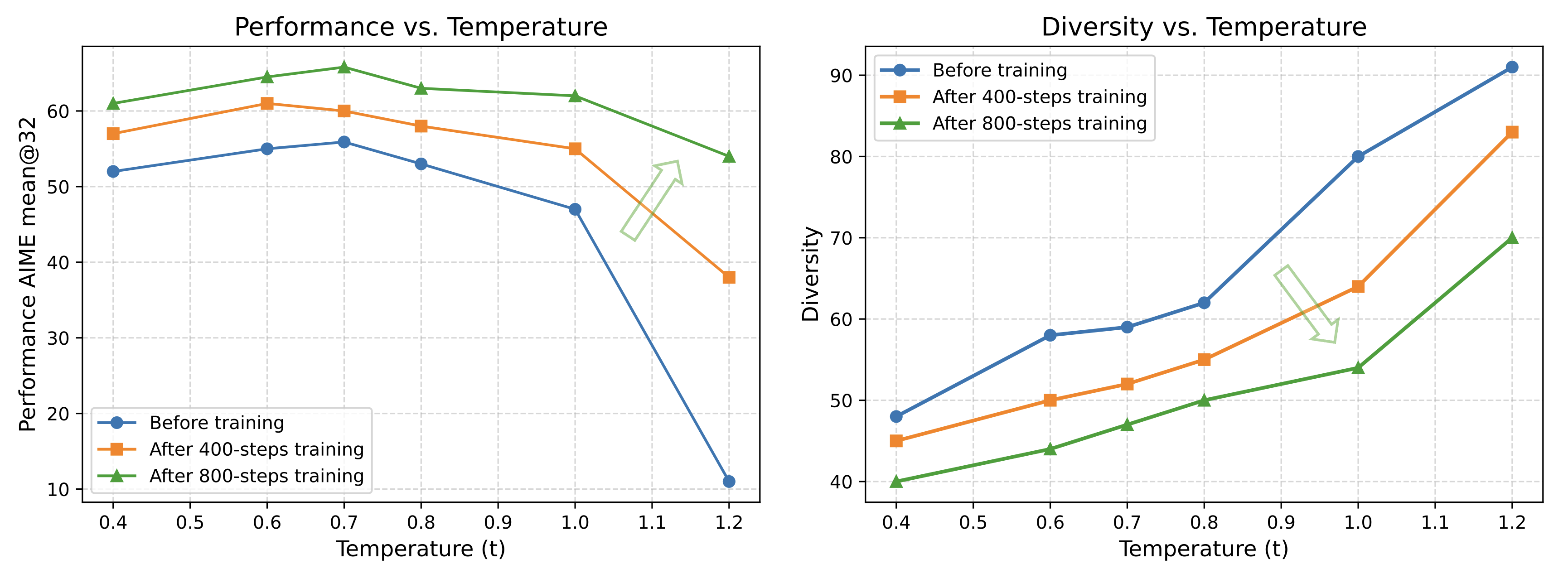
📌 Since the diversity of sample trajectories is critical for RL training, using the same sampling temperature throughout the training process can result in insufficient diversity at the later training stages and limit the potential for performance gains.
Therefore, we propose dynamically updating the temperature during RL training. As the model converges on high-quality patterns, we will increase the sampling temperature to encourage further exploration.
After each training stage, we will use a higher sampling temperature to maintain the model’s previous diversity score.
Specifically, we test various sampling temperatures and select the one that achieves the desired diversity score. Our experiments suggest setting the temperature interval based on the previous stage’s entropy decrease. If entropy decreases slightly, we recommend a 0.05 interval for the sampling temperatures. If entropy decreases significantly, we will use a larger interval. We show the sampling temperatures of each stage of Polaris in this Table:
| Stage-1 | Stage-2 | Stage-3 | |
|---|---|---|---|
Polaris-7B-Preview | 0.7 | 1.0 | 1.1 |
Polaris-4B-Preview | 1.4 | 1.45 | 1.5 |
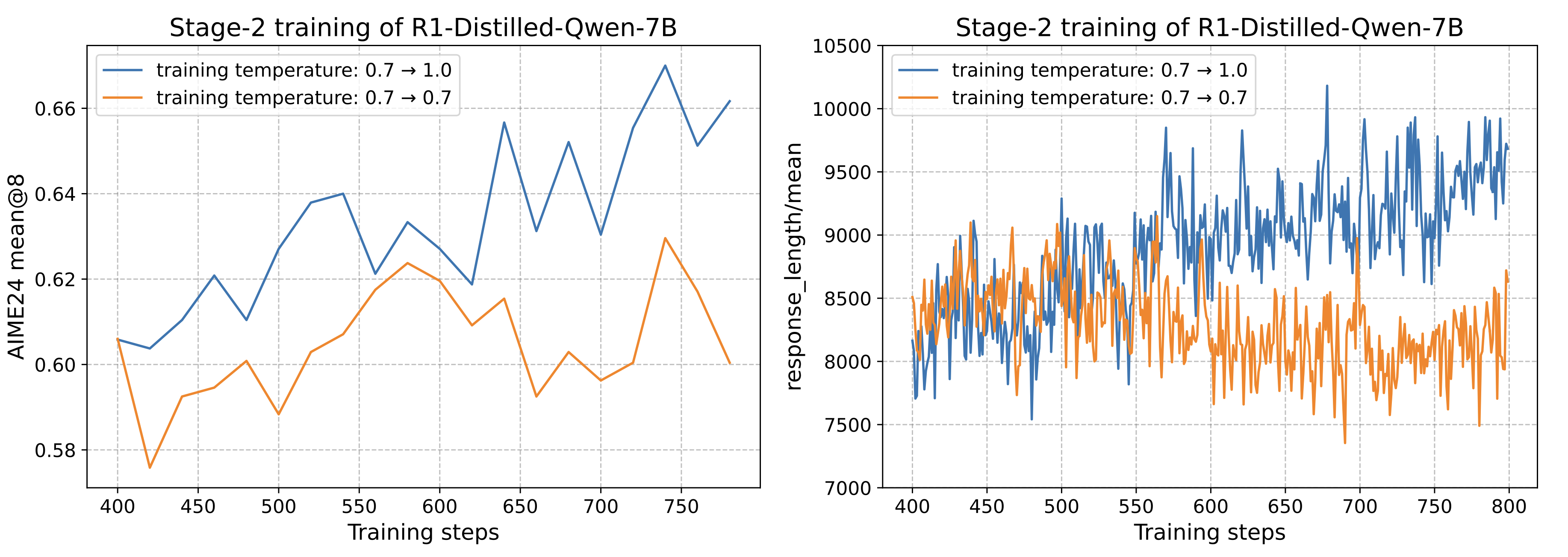
To verify the effectiveness of temperature increase, we conduct a baseline with the same temperature across the whole training. As we can see, the multi-stage with increased temperature leads to better RL training and further expanding the model’s thought depth by expanding the response length.
**3. Inference-Time Length Scaling
insufficient long-context training in RL stage
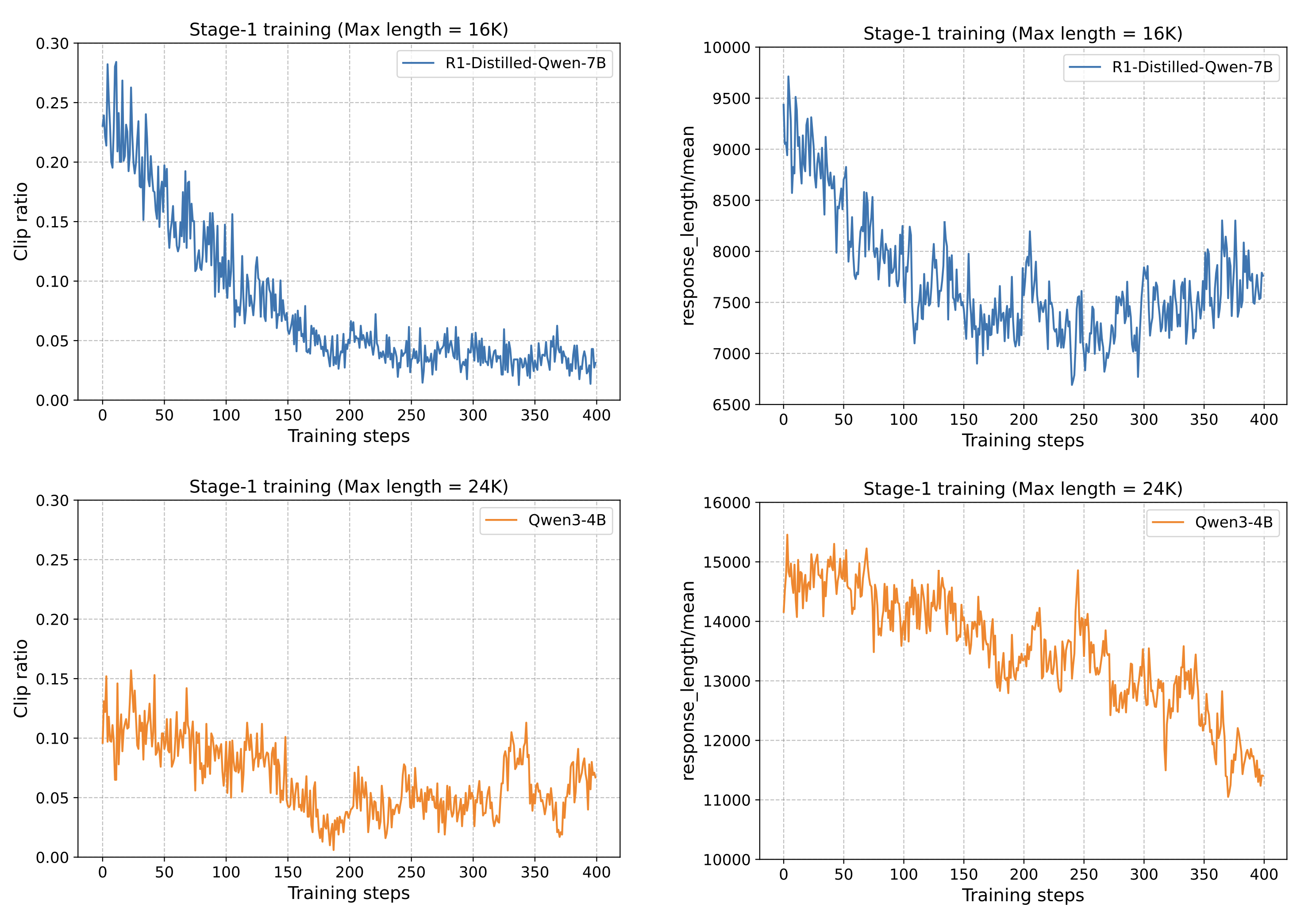
A significant challenge in developing advanced reasoning models is the cost of long-context training. For instance, our model, based on Qwen3-4B, has a pre-training context length of 32K. While we increase the maximum training length to 52K during RL, our experiments reveal a critical limitation. The clip_ratio, which measures the proportion of training samples that reach the maximum sequence length, remained below 10%. This indicates that very few samples are actually trained at the 52K length. During the RL training process, the inference time for rollouts often consumes a significant amount of resources. Within a single batch, if no additional optimizations are made, shorter samples must wait for longer samples to finish decoding, leading to wasted training time and resources. Therefore, it is not efficient to directly use a large training length. We also try some train-short, test-long methods to increase the inference length given limited training budgets.
Performance degradation beyond pre-training length
To quantify the effective Chain-of-Thought (CoT) length of Polaris-4B-Preview , we conduct an analysis using 60 problems from the AIME 2024/25 datasets. There are 32 rollouts for each problem (for a total of 1,920 rollouts) and grouped them by the length of the response:
- Short Rollouts Group: Responses with a length of less than 16K.
- Mid-Length Rollouts Group: Responses with a length between 16K and 32K.
- Long Rollouts Group: Responses with a length exceeding the 32K pre-training limit.
The Accuracy for each group is calculated using the following formula:
$\text{Accuracy} = \frac{\text{Number of Correct Rollouts}}{\text{Total Rollouts in Group}}$
The results were striking (blue bars). We observe a dramatic performance drop for responses in the Long Rollouts Group, which achieved an accuracy of only 26%.
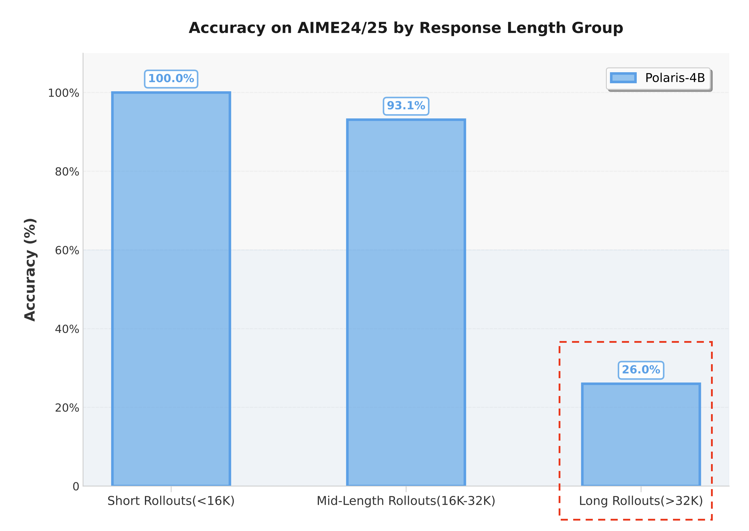
This finding supports our hypothesis: due to the inefficiencies of long-context RL training, the model struggles to generate effective and accurate long CoTs beyond its original pre-training length, even though the RL training length is set to 52K.
Training-free Length Extrapolation
To address this, we introduce length extrapolation technique in long reasoning traces generation, which follows the principle of “train shorter, test longer.” By adjusting the model’s Rotary Position Embeddings (RoPE), this method allows the model to maintain its performance on sequences longer than those seen during training, effectively compensating for insufficient long-context training.
For ease of implementation, we adopt the Yarn method with a scaling factor of 1.5. While Yarn recommends adjusting the attention temperature during extrapolation, we find that this modification—though beneficial for long-context retrieval tasks—is detrimental for generating long reasoning sequences.
  "rope_scaling": {
    "attn_factor": 1.0,
    "factor": 1.5,
    "rope_type": "yarn"
  }
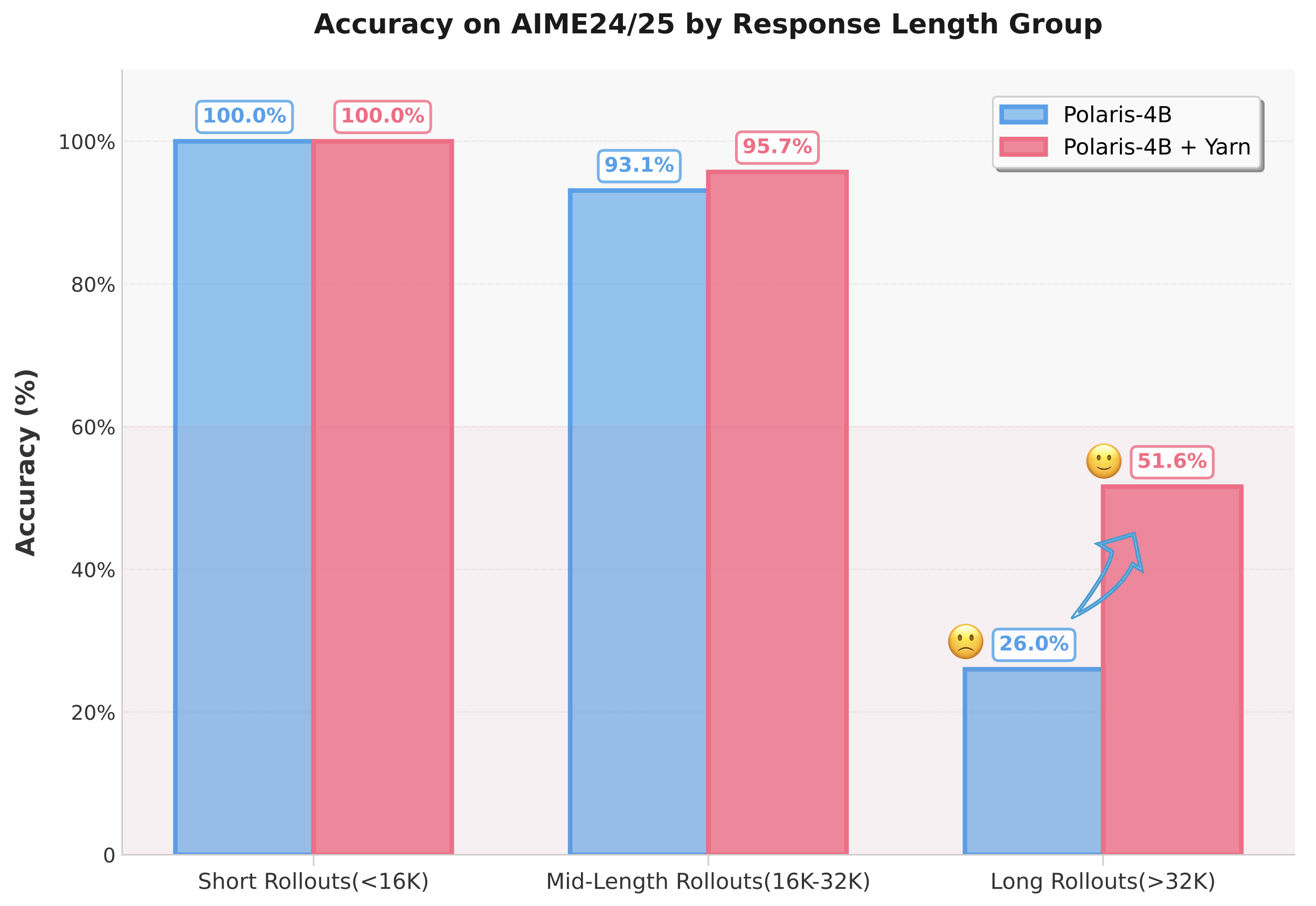
By applying Yarn at inference time—with no retraining required—we boost the accuracy on responses longer than 32K from 26% to over 50%!
This discovery suggests that CoT extrapolation is a powerful tool for the later stages of training advanced reasoning models, especially when increasing rollout length becomes unaffordable. We also note that the accuracy improvements are concentrated on the more difficult problems in the dataset.
Extrapolation Benefits Inference-Time Scaling
The graph below illustrates the inference-time scaling capabilities unlocked by Yarn on the AIME 24/25 datasets. The blue line represents Polaris-4B-Preview with Yarn, while the orange line shows the baseline performance without it.
As the chart demonstrates, Polaris-4B-Preview with Yarn (blue line) significantly outperforms its base model, Qwen3-4B, once the context length exceeds 48K. Its performance continues to grow as the length increases toward 96K. In contrast, the model without Yarn (yellow line) shows its performance plateauing after 64K with almost no further gains.
This confirms that applying an extrapolation technique like Yarn at inference time unlocks the model’s potential to scale its reasoning abilities to much longer contexts, overcoming the limitations imposed by practical RL training constraints.

4. Exploration Efficiency
The success of long CoT training hinges on efficient exploration at the frontier of reward sparsity. In Polaris, exploration efficiency is enhanced through multi-stage training, accompanied with techniques that address response-level and sample reward sparsity. Specifically, we found that:
- the previously proposed “Think Shorter, then Longer” paradigm does not generalize to all reasoning models; directly training with longer responses can often yield better performance;
- dynamical sampling can be done easy with the proposed Rollout Rescue Mechanism and Intra-Batch Informative Substitution techniques.
Multi-Stage Training
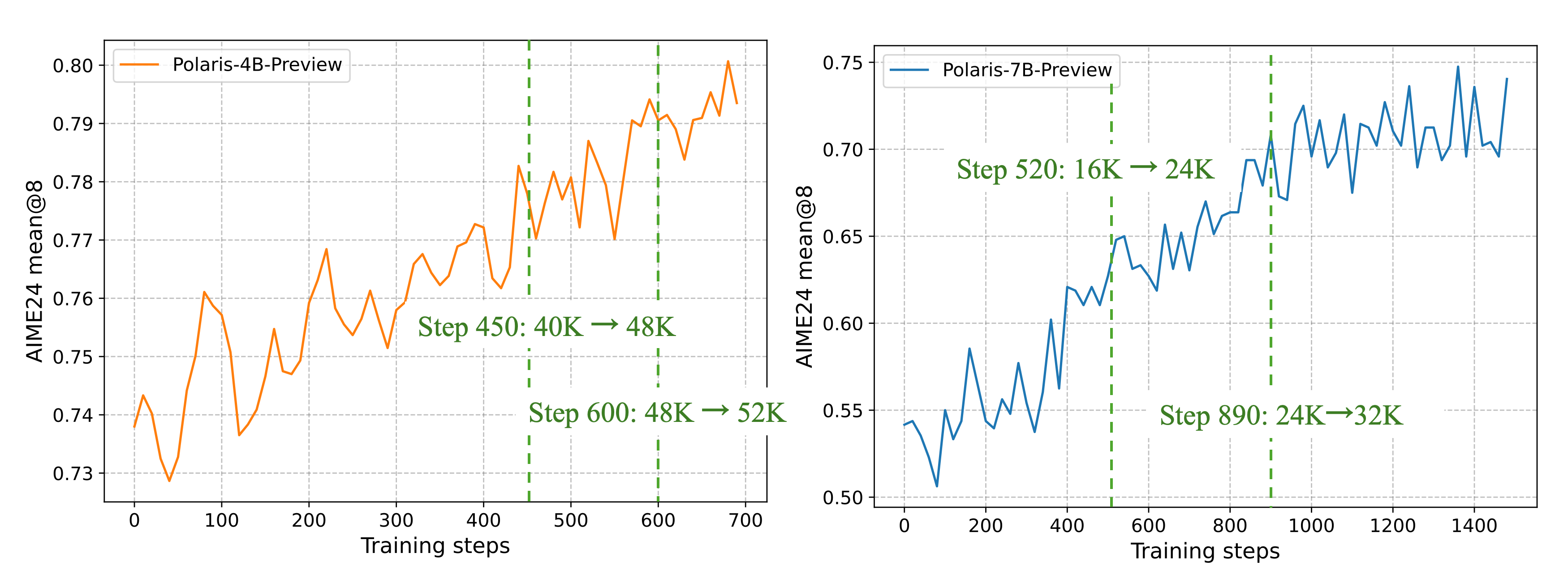
One of the biggest challenges in optimizing long CoT models with RL is the excessively long output, which results in slow training. To improve training efficiency, we incorporate multi-stage training in all our released models. Specifically, we use shorter context windows in earlier stages. Once the model’s performance converges, we increase the length of the context windows in the next stage.
Is “Think Shorter, then Longer” necessary?
While effective, for multi-stage training it is critical to select the appropriate response length at the first stage:
- Not all models are both equally token-efficient: We found that training at a small response length works well for
DeepSeek-R1-Distill-Qwen-7Bbut not forQwen3-4B. Specifically, we observe drastic performance drop forQwen3-4Beven at a response length of 24K and response clip ratio of <15%. Such performance degeneration is irreversible at later stages.
- It is usually safer to directly allow the model to “think longer” from the beginning: For
Qwen3-4B, we observed steadily increasing performance with a 40K response length from scratch, in stark contrast with 24K and 24K→40K schemes.
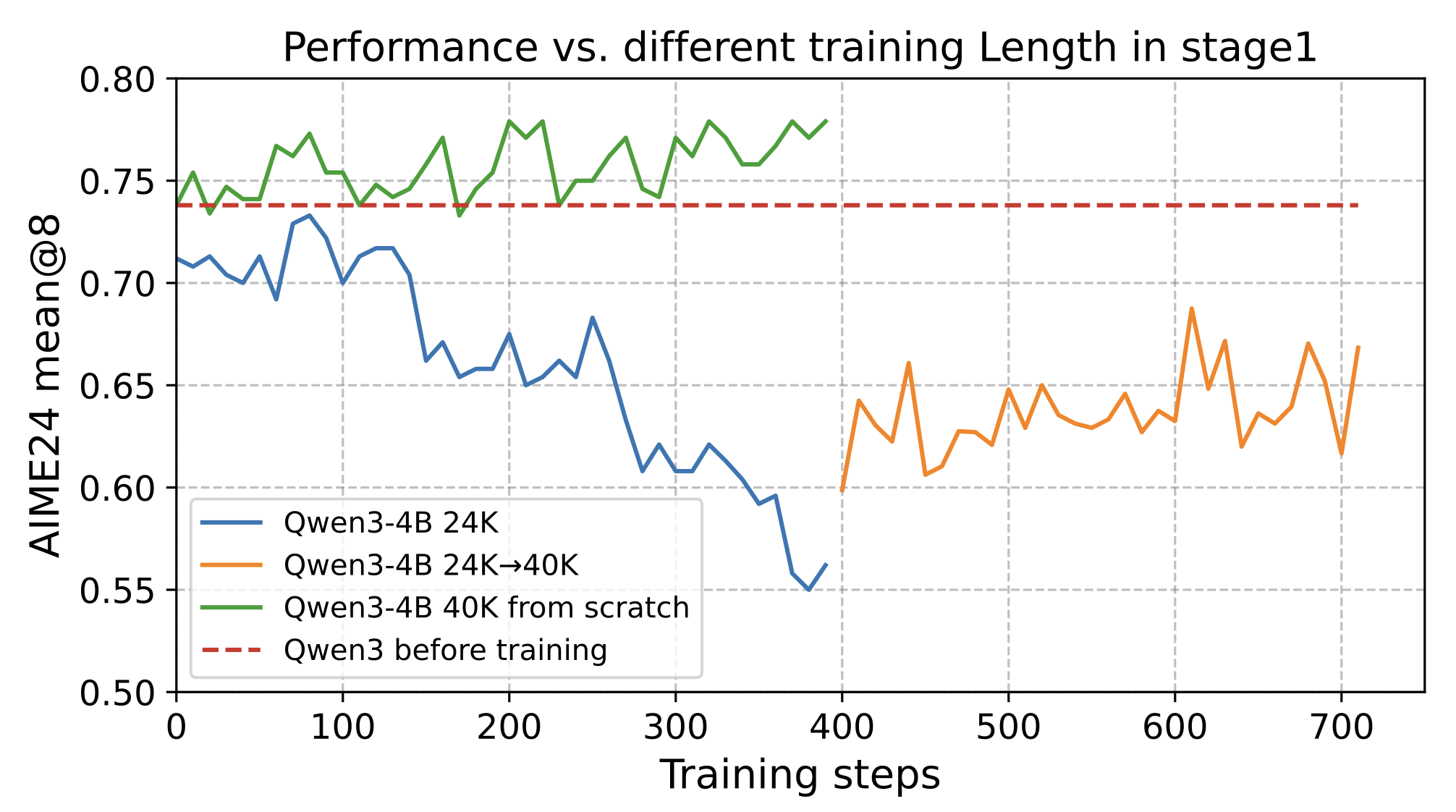
Takeaway: When computational resources allow, start directly with the maximum decoding length suggested by the official repository.
Rollout Rescue Mechanism
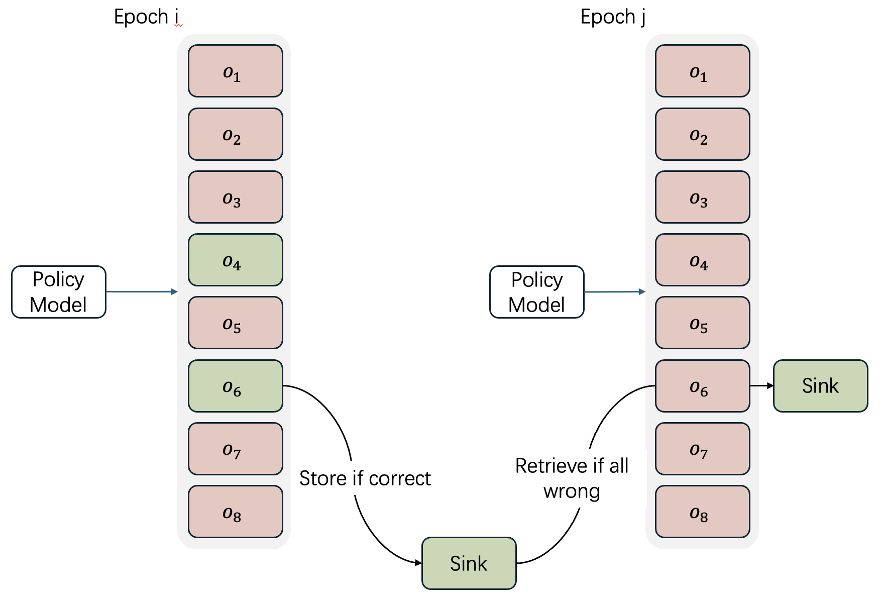
POLARIS uses a small rollout size (8) for cost savings, but this raises the chance of zero-reward batches on hard prompts. To balance positive examples with minimal engineering, we maintain a per-example offline buffer (“sink”):
- If all 8 rollouts fail (accuracy 0/8) and a correct rollout was observed in earlier epochs, store that response in the sink (evicting the previous one).
- In later epochs, whenever a new batch yields 0/8 for that example, randomly swap one failed rollout with the buffered response.
This lightweight strategy reduces zero-reward data dramatically and speeds up convergence, without retry loops.
Intra-Batch Informative Substitution
In GRPO, examples with all-correct or all-incorrect rollouts produce no advantage. Rather than complex dynamic sampling, we apply a simple in-batch swap:
- Within each batch, select samples that have a mix of correct and incorrect rollouts (nonzero advantage).
- Randomly duplicate these informative samples to replace those that yield zero advantage.
This ensures every training example contributes a learning signal, matching DAPO’s benefits but requiring only a few tensor index operations—no extra rollouts or data-pipeline changes.
5. From DAPO and GRPO+
We’ve incorporated several key strategies from DAPO and GRPO+ into our training process for the following reasons:
- No Entropy Loss (from GRPO+): We remove the entropy loss term to prevent training instability. While intend to encourage exploration, we note it can cause entropy to grow uncontrollably, leading to a training collapse. Our primary motivation is to ensure a more stable and reliable training process.
- No KL Loss (from DAPO): We eliminate the KL loss to allow our model to explore beyond the constraints of the original SFT model. This also speeds up training, as we no longer need to compute log probabilities for a reference model.
- Clip High (from DAPO): We increase the upper clipping bound in the surrogate loss function to encourage more aggressive exploration. This adjustment helps stabilize entropy and has been shown to improve model performance by allowing the policy to take larger, more beneficial update steps.
6. Reward Function
The reward function used in this work is the same as DeepscaleR, we employ an Outcome Reward Model (ORM) which returns:
-
1- If the LLM’s answer passes basic LaTeX/Sympy checks. -
0- If the LLM’s answer is incorrect or formatted incorrectly (e.g. missing<think>,</think>delimiters).
Evaluation
Our model needs to use a higher sampling temperature and a longer response length than Qwen3; all other settings are the same. For AIME24 and AIME25, we report the average performance of 32 runs.
    sampling_params = SamplingParams(
        temperature=1.4,
        top_p=1.0,
        top_k=20,
        max_tokens=90000
    )
example input: <|im_start|>user\nEvery morning Aya goes for a $9$-kilometer-long walk and stops at a coffee shop afterwards. When she walks at a constant speed of $s$ kilometers per hour, the walk takes her 4 hours, including $t$ minutes spent in the coffee shop. When she walks $s+2$ kilometers per hour, the walk takes her 2 hours and 24 minutes, including $t$ minutes spent in the coffee shop. Suppose Aya walks at $s+\\frac{1}{2}$ kilometers per hour. Find the number of minutes the walk takes her, including the $t$ minutes spent in the coffee shop. Let's think step by step and output the final answer within \\boxed{}.<|im_end|>\n<|im_start|>assistant\n
The evaluation scripts based on Verl have been released on our GitHub. You can also use your own scripts for testing, but please note: our model’s output length has been significantly boosted. If your max response length is set too small, the performance may not even reach the level of the original Qwen3-4B due to the truncation mechanism. Therefore, please ensure the testing length is at least 64K. The graph showing performance changes with response length is available in the “Inference-Time Length Scaling” section.
| Models | AIME24 avg@32 | AIME25 avg@32 | Minerva Math avg@4 | Olympiad Bench avg@4 | AMC23 avg@8 |
|---|---|---|---|---|---|
DeepScaleR-1.5B | 43.1 | 27.2 | 34.6 | 40.7 | 50.6 |
Qwen3-1.7B | 48.3 | 36.8 | 34.9 | 55.1 | 75.6 |
POLARIS-1.7B-Preview | 66.9 | 53.0 | 38.9 | 63.8 | 85.8 |
Deepseek-R1-Distill-Qwen-7B | 55.0 | 39.7 | 36.7 | 56.8 | 81.9 |
AReal-boba-RL-7B | 61.9 | 48.3 | 39.5 | 61.9 | 86.4 |
Skywork-OR1-7B-Math | 69.8 | 52.3 | 40.8 | 63.2 | 85.3 |
POLARIS-7B-Preview | 72.6 | 52.6 | 40.2 | 65.4 | 89.0 |
Deepseek-R1-Distill-Qwen-32B | 72.6 | 54.9 | 42.1 | 59.4 | 84.3 |
qwen3-32B | 81.4 | 72.9 | 44.2 | 66.7 | 92.4 |
qwen3-4B | 73.8 | 65.6 | 43.6 | 62.2 | 87.2 |
POLARIS-4B-Preview | 81.2 | 79.4 | 44.0 | 69.1 | 94.8 |
Citation
@misc{Polaris2025,
    title = {POLARIS: A Post-Training Recipe for Scaling Reinforcement Learning on Advanced Reasoning Models},
    url = {https://hkunlp.github.io/blog/2025/Polaris},
    author = {An, Chenxin and Xie, Zhihui and Li, Xiaonan and Li, Lei and Zhang, Jun and Gong, Shansan and Zhong, Ming and Xu, Jingjing and Qiu, Xipeng and Wang, Mingxuan and Kong, Lingpeng}
    year = {2025}
}